Using Machine Learning to Peek Inside the Minds of NFL Coaches

Unlike baseball and basketball where analytics is already being used, data analytics for football is still in its nascent phase. The race is now on to figure out how to use that data better than anyone else. With far fewer games per season than baseball and many variables, football brings up a whole new set of points to analyze, and there is a huge advantage to digging into this new trove of information. 

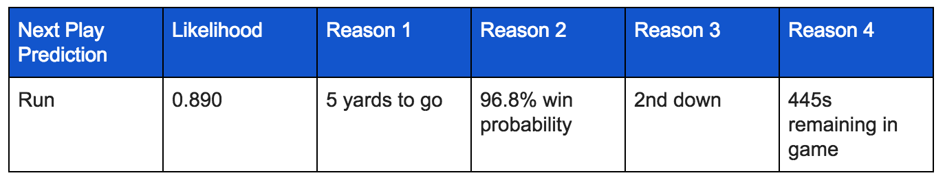
What if I told you it was possible to predict what type of play your opponent is likely to run? Imagine as a head coach, after every play, your AI team delivers a simple report like this. How else could this information be valuable?  Maybe it could be used to uncover predictable tendencies in your own team? Or maybe even help fans to win bigger in Las Vegas?

Even though AI adoption in the NFL is relatively low, NFL organizations are increasingly turning to advanced analytics and machine learning to extract insights and make decisions. Teams are starting to investigate and develop AI solutions that rely less on gut and more on the combination of expertise, statistics and data. This year, the NFL started sharing advanced statistics based on location data, which allows tracking player movement.

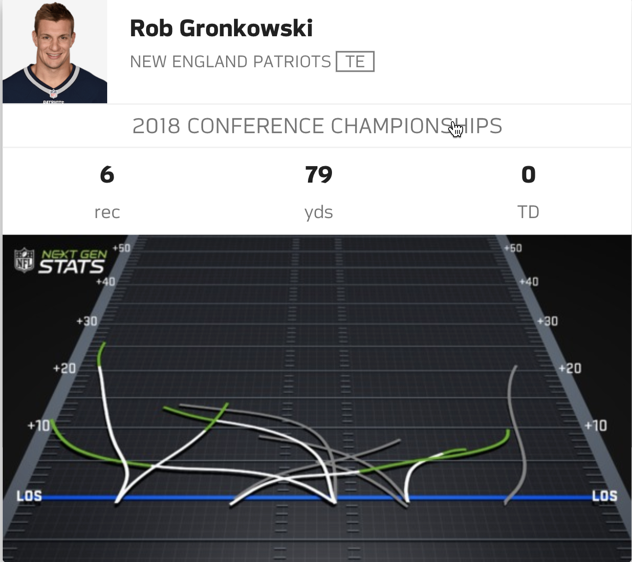
Source: https://nextgenstats.nfl.com/

In this simple example, I’d like to demonstrate how using DataRobot can help teams make better tactical decisions in between plays. Imagine yourself as the leading data scientist for a professional NFL team in charge of developing and deploying real-time in game models. Let’s say that the General Manager asks you and your team to see if you can analyze opponent tendencies and develop a model to predict whether the next play will be a run or a pass. The GM plans to use this model to augment and speed up the decision-making process for personnel, schemes, and packages.

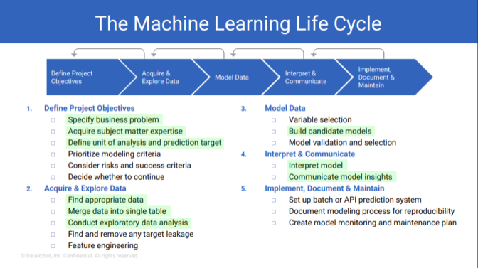
DataRobot Model Development Cycle

DataRobot recommends following an iterative development cycle for building models. This cycle improves performance and shortens the development time substantially. While I don’t intend to go through the entire cycle in this post, I want to highlight a portion of this cycle with the objective of delivering a minimally viable model (MVM) with insights and plans for future iterations.

The Data

The dataset contains play-by-play data for each regular season game from 2009-2018.  In the original dataset, there were 400K rows and 255 features. The goal of the exercise is to deliver an MVM, so a simple feature selection model was built to reduce the number of features to 50.  Below is a quick summary of the input data of the top 10 features, plus the target, from the automated exploratory data analysis (EDA) capabilities in DataRobot.

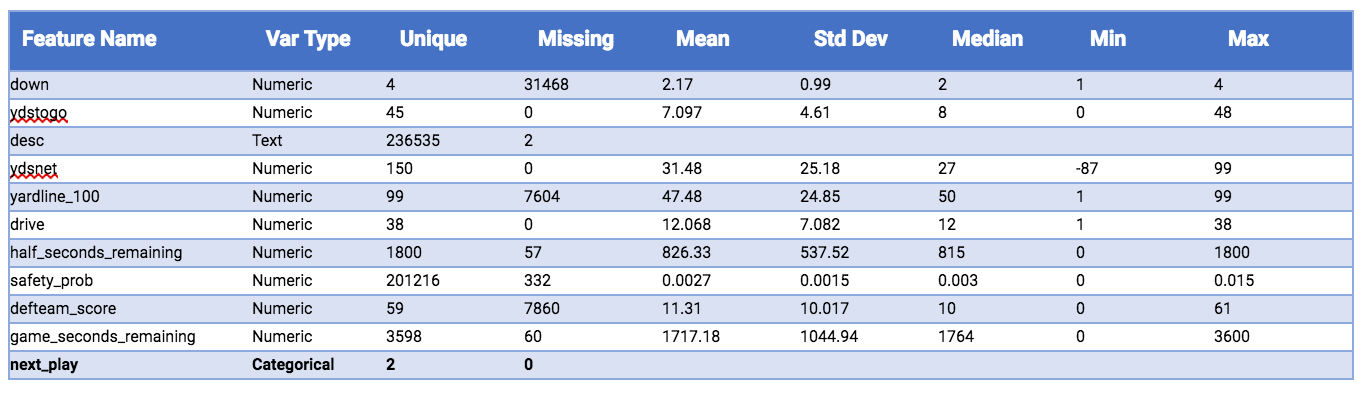
DataRobot automates the generation of EDA tables, which give you quick insights into the training data. For every feature in the input data, you learn about the number of unique values, missing data, data type, and a set of descriptive statistics if data type is numeric.

Modeling using DataRobot’s Automated Machine Learning

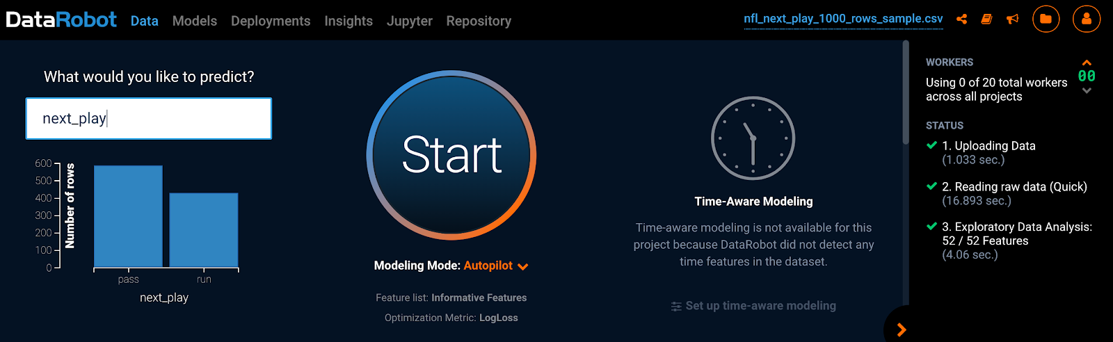
Once you upload the data, select the target, “next_play,” and hit start. It’s that easy to build many models in minutes!

Model Performance

DataRobot’s Leaderboard automatically scores and sorts the challenger models on the out-of-sample validation data. Here is a snapshot of the top few models.

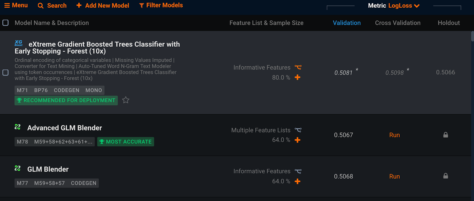
The top performing model is the eXtreme Gradient Boosted Trees Classifier with Early Stopping – Forest (10x) with a log loss of 0.5081.

Insights

Let’s take a look at what we learned in our first iteration or MVM.

Model Evaluation

When quick decisions are paramount, sometimes simple models are best. DataRobot includes the ability to build a RuleFit Classifier. This model constructs classification models as an ensemble of simple rules + coefficients for each rule. RuleFit models have demonstrated competitive performance and simple rules that are easy to implement and interpret.  Here are some hotspots detected using the RuleFit classifier:

• When it’s 1st or 2nd down and the yards to go is between 6 and 10 yards, there is a 79% chance that the next play is run.

• When the time remaining in either half is less than 118s, there is a 17% chance that the next play is a run.

Individually, these rules are not surprising, but in combination they can be quite powerful and easy to implement.

Classification Accuracy and The Confusion Matrix

DataRobot automatically calculates a number of the most critical statistics for measuring the real-world performance of a classification model, including accuracy, sensitivity and precision.

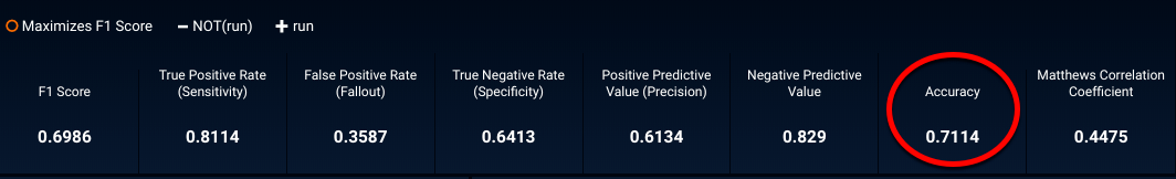
For the MVM, the model predicts the correct play 71% of the time. This is not bad for an MVM. Perhaps in subsequent iterations of the model, the accuracy can climb well into the 80’s.

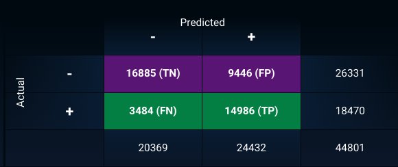
In subsequent iterations, balancing the impact of false positives, when the model predicts a run and the actual play is a pass with false negatives, when the model predicts a pass and the actual play is a run, will be important. For now, let’s continue to see how well the MVM performs.

ROC Curve and Prediction Distribution Analysis

The ROC (Receiver Operating Characteristic) curve and the prediction distribution histograms are nice tools that help you analyze the performance, robustness, and set thresholds to choose whether the next play is a pass or a run.

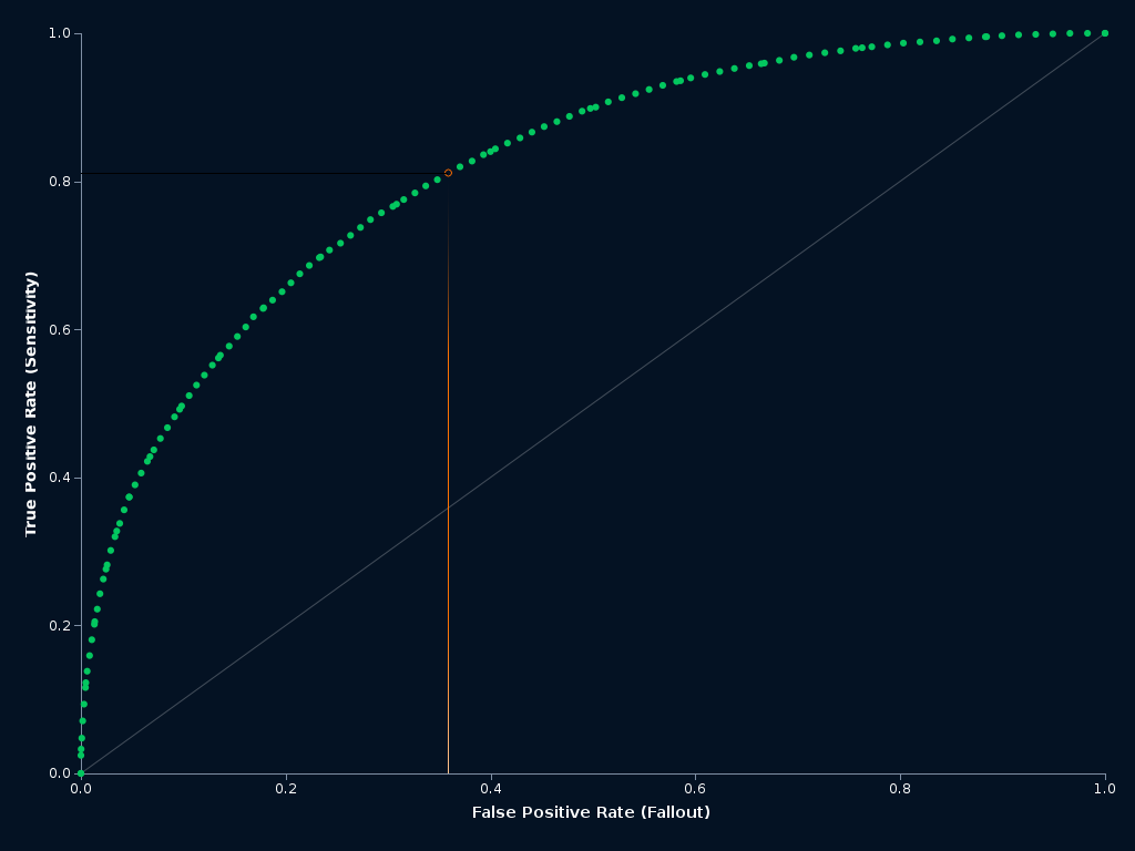
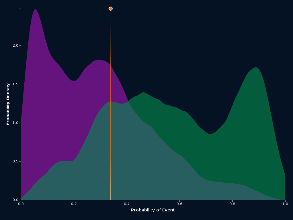
In this case, the event is a run. The green distribution (right) represents all the runs and the purple distribution represents all the passes. The orange line is the optimal threshold, chosen to maximize the balance between precision and recall. There is significant overlap in the distributions, which means, at times, it will be difficult to predict the next play.

Feature Effects

Analyzing individual features and the effect they have on the tendency to call run or pass plays can be very insightful. Sometimes feature effects, which uses partial dependence (PD) to measure, can either reinforce your intuition or call it into question. A partial dependence plot illustrates the marginal effect that a given feature has on the predicted value. A partial dependence plot can show whether the relationship between the target and a feature is linear, monotonous or more complex.  I took a look at the top handful of features to do a deeper dive.

Yards to go (yrdstogo)

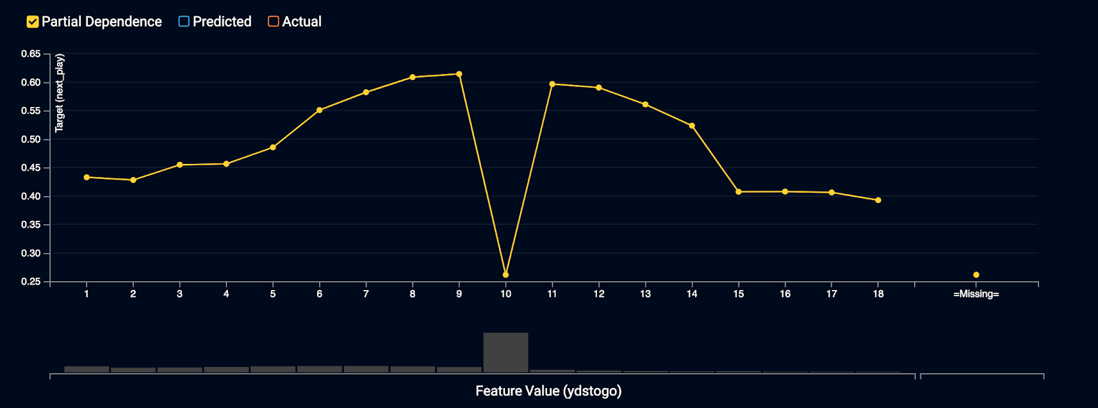
For yards to go, you see some interesting trends as the distance needed to get a first down increases. Interestingly enough, the fraction of time a run is called generally increases from 1-9 yards. There is a dip when yrdstogo = 10.  Every series starts with a first and 10, but if you throw an incomplete pass or don’t gain any yards, the yrdstogo still equals 10. The mode of the data is also at 10. The partial dependence plot is picking up on the relationship between yrdstogo and run frequency, but is conflating the marginal effect of all the other features, like down. This insight begs a deeper dive, which we may touch in subsequent iterations.

Down (down)

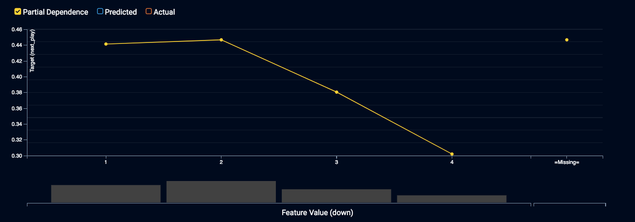
Analyzing the PD plot for down, it shows the marginal impact (holding all other features constant) that down has on the likelihood that a run will be called. Not surprisingly, the likelihood of a run is highest on 1st and 2nd down, but I was surprised at the marginal effect when it is 4th down. I expected the likelihood of a run to be much higher as I assumed most 4th down plays that aren’t punts or field goals to be 4th and short. This effect must be a combination of desperation pass plays, end of half or game play calls that are low risk and those 4th and short plays, which will likely diminish the likelihood of a run.

Touchdown Probability (td_prob)

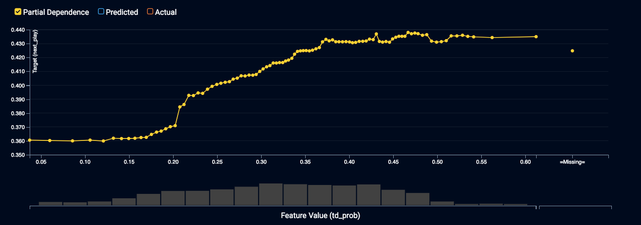
During goal line situations when the probability of a touchdown is highest, the likelihood of a run increases. The marginal effect of td_prob on the likelihood of a run shows a positive relationship that levels out at about 44%.

Conclusions

With so much on the line, NFL teams are searching for any edge they can get on the competition. Piggybacking off of the sports analytics revolution that has occurred in other sports (e.g. Moneyball in baseball and the reliance on the 3pt shot in the NBA), NFL teams are increasingly likely to look for an edge in their data. Sports analytics will continue to change professional sports, with AI playing a huge role in the change. In this simple example, we demonstrate the power of machine learning to help make real-time decisions. The MVM utilizing historical in game data yields a model that has the ability to predict the next play at 71% accuracy.  Here is a snapshot of predictions on the holdout data.

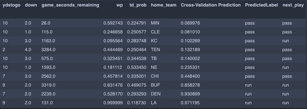
At the extremes of the predicted probability of a run (Cross-Validation Prediction), the MVM does quite well, but the real power of the model will be in uncovering the tendencies when the outcome is uncertain.

As a start, the MVM looks promising and during subsequent iterations, improvement is expected. Some possible next steps would be to engineer new features like team run probabilities per down or situationally aware features. I will also like to test DataRobot’s time series functionality to see if I can build an even more powerful model.

About the author

Benjamin Miller

Customer Facing Data Scientist at DataRobot

Ben Miller is a Customer Facing Data Scientist at DataRobot with a strong background in data science, advanced technology, and engineering. Ben is a machine learning professional with demonstrable skills in the area of multivariable regression, classification, clustering, predictive analytics, active learning, natural language processing, and algorithm R&D. He has scientific training and application in disparate industries including; biotechnology, life sciences, pharmaceutical, environmental, human resources, banking, and media.

Meet Benjamin Miller